The discovery of oil and gas fields is the main goal of seismic exploration. Actually, most of today’s industrial activities still rely on hydrocarbons. However, oil exploration is an expensive, high-risk operation, and the oil companies want to be sure that it is worth drilling a new oil well. Thus, it becomes mandatory to locate the position and extension of the reservoirs with a high accuracy.
Visible surface features such as oil or natural gas seeps, pockmarks (underwater craters caused by escaping gas) provide basic evidence of hydrocarbon generation (be it shallow or deep in the earth). However, most exploration depends on highly sophisticated technologies to detect and determine the extent of these deposits using exploration geophysics.
Therefore, several numerical techniques have been developed in order to help locate hydrocarbons reservoirs.
We approach the problem through a Full Waveform Inversion (FWI) – based method. The FWI method aims at recovering the velocity profile of the field, and in turn the rock properties, by solving an inverse problem associated with the wave equation.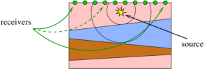 In particular, a functional that accounts for the misfit between recorded and computed data is minimized.
Unfortunately, this inverse problem is, in general, not well-posed, because different velocity profiles of the field can lead to (almost) the same recorded data. The seismic inversion is actually based on seismic reflection data, which are collected in seismic surveys (Figure in the right).
In order to try and improve the performance of the classical FWI method, i.e., its high sensitivity to the initial velocity guess and the above-mentioned ill posedness, we propose a method that suitably combines data obtained by shooting several sources. Moreover, while in the classical FWI method a Tikhonov regularization is usually added to the misfit functional, we use a Total Variation (TV) regularization term. This should take into account the discontinuities of the velocity profile to be recovered in a more accurate way.
Numerical example
Data:
- Sources position: z=30m , x=[75 133 192 258 317 383 442] m
- Receivers position: 8.3 m apart, on the surface (first cell)
- Source(t) = 10 sin(16 pi t) MPa /km^2
- TV constant = 1e-8
- Dx = Dz = 8.3m
- Dt = 1ms
- Tf = 0.5s
Discretization: finite difference in space + leap-frog in time
Optimization: Barzilai-Borwein method
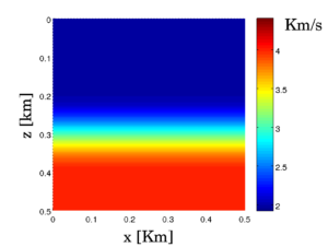
Initial guess for the FWI procedure.
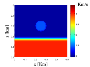
Reference solution.
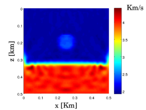
Reconstructed profile with no regularization.
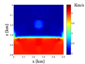
Reconstructed profile with TV regularization.